More on the algorithms
Algorithms
Baseline
We drew from Lignos (2012) the excellent idea of drawing baselines by cutting with a given probability. Using this insight, you can draw four baselines:
the random baseline randomly labels each syllable boundary as a word boundary with a probability P = 0.5. If no P is specified by the user, this is the one that is ran by default.
the utterance baseline treats every utterance as a single word, so P = 0.
the basic unit baseline labels every phone (or syllable) boundary as a word boundary, so P = 1,
Finally, the user can also get oracle baseline with a little bit more effort. You can run the stats function to get the number of words and the number of phones and syllables. Then divide number of phones by number of words to get the probability of a boundary in this data set when encoded in terms phones, let us call it PP. You then set the parameter P = PP in the input prepared in terms of phones. Or, if you are preparing your corpus tokenized by syllables, use PS= number of syllables / number of words.
For more inforamtion, see Lignos, C. (2012). Infant word segmentation: An incremental, integrated model. In Proceedings of the West Coast Conference on Formal Linguistics (Vol. 30, pp. 13-15).
Diphone Based Segmenter (DiBS)
A DiBS model is any model which assigns, for each phrase-medial diphone, a value between 0 and 1 inclusive, representing the probability the model assigns that there is a word-boundary between the two phones. In practice, these probabilities are mapped to hard decisions (break or no break).
Making these decisions requires knowing the chunk-initial and chunk-final probability of each phone, as well as all diphone probabilities; and additionally the probability of a sentence-medial word boundary. In our package, these 4 sets of probabilities are estimated from a training corpus also provided by the user, where word boundaries are marked. Please note we say “chunk-initial and chunk-final” because the precise chunk depends on the type of DiBS used, as follows.
Three versions of DiBS are available. DiBS-gold is supervised in that “chunks” are the gold/oracle words. It is thus supposed to represent the optimal performance possible. DIBS-phrasal uses phrases (sentences) as chunks. Finally, DIBS-lexical uses as chunks the components of a seed lexicon provided by the user (who may want to input e.g. high frequency words, or words often said in isolation, or words known to be known by young infants).
The probability of word boundary right now is calculated in the same way for all three DiBS, and it’s the actual gold probability (i.e., the number of words minus number of sentences, divided by the number of phones minus number of sentences). Users can also provide the algorithm with a probability of word boundary calculated in some other way they feel is more intuitive.
DiBS was initially designed with phones as basic units. However, for increased flexibility we have rendered it possible to use syllables as input.
For more information, see Daland, R., & Pierrehumbert, J.B. (2011). Learning diphone-based segmentation. Cognitive science, 35(1), 119–155. You can also view an annotated example produced by Laia Fibla on https://docs.google.com/document/d/1tmw3S-bsecrMR6IokKEwR6rRReWknnbviQMW2o0D5rM/edit?usp=sharing.
Transitional probabilities
In conceptual terms, we can say that such algorithms assume that infants are looking for words defined as internally cohesive phone/syllable sequences, i.e. where the transitional probabilities between the items in the sequence are relatively high. Our code was provided by Amanda Saksida, where transitional probabilities (TPs) can be calculated in three ways:
Forward TPs for XY are defined as the probability of the sequence XY divided by the probability of X;
Backward TPs for XY are defined as the probability of the sequence XY divided by the probability of Y;
Mutual information (MI) for XY are defined as the probability of the sequence XY divided by the product of the two probabilities (that of X and that of Y).
As to what is meant by “relatively high”, Saksida’s code flexibly allows two definitions. In the first, a boundary is posted when a relative dip in TP/MI is found. That is, given the syllable or phone sequence WXYZ, there will be a boundary posited between X and Y if the TP or MI between XY is lower than that between WX and YZ. The second version uses the average of the TP/MI over the whole corpus as the threshold. Notice that both of these are unsupervised: knowledge of word boundaries is not necessary to compute any of the parameters.
TPs was initially designed with syllables as basic units. However, for increased flexibility we have rendered it possible to use phones as input.
For more information, see Saksida, A., Langus, A., & Nespor, M. (2017). Co‐occurrence statistics as a language‐dependent cue for speech segmentation. Developmental science, 20(3). You can also view an annotated example produced by Georgia Loukatou on https://docs.google.com/document/d/1RdMlU-5qM22Qnv7u_h5xA4ST5M00et0_HfSuF8bbLsI/edit?usp=sharing
Phonotactics from Utterances Determine Distributional Lexical Elements (PUDDLE)
This algorithm was proposed by Monaghan and Christiansen (2010), who kindly shared their awk code with us. It was reimplemented in python in this package, in which process one aspect of the procedure may have been changed, as noted below.
Unlike local-based algorithms such as DiBS and TPs, PUDDLE takes larger chunks – utterances – and breaks them into candidate words. The system has three long-term storage buffers: 1. a “lexicon”, 2. a set of onset bigrams, and 3. a set offset bigrams. At the beginning, all three are empty. The “lexicon” will be fed as a function of input utterances, and the bigrams will be fed by extracting onset and offset bigrams from the “lexicon”. The algorithm is incremental, as follows.
The model scans each utterance, one at a time and in the order of presentation, looking for a match between every possible sequence of units in the utterance and items in the “lexicon”.
We can view this step as a search made by the learner as she tries to retrieve words from memory a word to match them against the input. _The one change we fear our re-implementation may have caused is that the original PUDDLE engaged in a serial search in a list sorted by inverse frequency (starting from the most frequent items), whereas our search is not serial but uses hash tables._ In any case, if, for a considered sequence of phones, a match is found, then the model checks whether the two basic units (e.g. phones) preceding and following the candidate match belong to the list of beginning and ending bigrams. If they do, then the frequency of the matched item and the beginning and ending bigrams are all increased by one, and the remainders of the sentence (with the matched item removed) are added to the “lexicon”. If a substring match is not found, then the utterance is stored in the long-term “lexicon” as it is, and its onset and offset bigrams will be added to the relevant buffers.
In our implementation of PUDDLE, we have rendered it more flexible by assuming that users may want to use syllables, rather than phones, as basic units. Additionally, users may want to set the length of the onset and offset n-grams. Some may prefer to use trigrams rather than biphones; conversely, when syllables are the basic unit, it may be more sensible to use unigrams for permissible onsets and offsets. Our implementation is, however, less flexible than the original PUDDLE in that the latter also included a parameter for memory decay, and for word-internal sequence cohesiveness.
For more information, see Monaghan, P., & Christiansen, M. H. (2010). Words in puddles of sound: modelling psycholinguistic effects in speech segmentation. Journal of child language, 37(03), 545-564. You can also view an annotated example produced by Alejandrina Cristia on https://docs.google.com/document/d/1OQg1Vg1dvbfz8hX_GlWVqqfQxLya6CStJorVQG19IpE/edit?usp=sharing
Adaptor grammar
In the adaptor grammar framework, parsing a corpus involves inferring the probabilities with which a set of rewrite rules (a “grammar”) may have been used in the generation of that corpus. The WordSeg suite natively contains one sample grammar, the most basic and universal one, and it is written in a phonetic alphabet we have used for English. Users should use this sample to create their own and/or change extant ones to fit the characteristics of the language they are studying (see https://github.com/alecristia/CDSwordSeg/tree/master/algoComp/algos/AG/grammars for more examples).
In the simplest grammar, included with the WordSeg suite, there is one rewrite rule stating that words are one or more basic units, and a set of rewrite rules the spell out basic units into all of the possible terminals. Imagine a simple language with only the sounds a and b, the rules would be:
Word –> Sound (Sound)
Sound –> a
Sound –> b
A key aspect of adaptor grammar is that it can also generate subrules that are stocked and re-used. For instance, imagine “ba ba abab”, a corpus in the above-mentioned simple language. As usual, we remove word boundaries, resulting in “babaabab” as the input to the system. A parse of that input using the rules above might create a stored subrule “Word –> ba”; or even two of them, as the system allows homophones. The balance between creating such subrules and reusing them is governed by a Pittman-Yor process, which can be controlled by the WordSeg using by setting additional parameters. For instance, one of this parameters, often called “concentration” determines whether subrules are inexpensive and thus many of them are created, or whether they are costly and therefore the system will prefer reusing rules and subrules rather than creating new ones.
The process of segmenting a corpus with this algorithm will in fact contain three distinct subprocesses. The first, as described above, is to parse a corpus given a set of rules and a set of generated subrules. This will be repeated a number of times (“sweeps”), as sometimes the parse will be uneconomical or plain wrong, and therefore the first and last sweeps in a given run will be pruned, and among the rest one in a few will be stored and the rest discarded.
The second subprocess involves applying the parses that were obtained in the first subprocess onto the corpus again, which can be thought of as an actual segmentation process. Remember that in some parses of the “ba ba abab” corpus (inputted as “babaabab”), the subrule “Word –> ba” might have been created 0, 1, or 2 times. Moreover, even if we ignore this source of variation, the subrules may be re-used or not, thus yielding multiple possible segmentations (“baba abab” with no subrule, “ba ba a ba b” with one “Word –> ba” subrule or the same with 3 “Word –> ba” subrules, etc.)
The third and final subprocess involves choosing among these alternative solutions. To this end, Minimum Bayes Risk is used to find the most common sample segmentations.
As this description shows, there are many potential free parameters, some that are conceptually crucial (concentration) and others that are closer to implementation (number of sweeps). By default, all of these parameters are set to values that were considered as reasonable for experiments (on English, Japanese, and French adult and child corpora) running at the time the package started emerging, and that we thus thought would be a fair basis for other general users. The full list can be accessed by typing wordseg-ag –h. The following is a selection based on what is often reported in adaptor grammar papers:
number of runs: 8
number of sweeps per run: 2000
number of sweeps that are pruned: 100 at the beginning and end, 9 in every 10 in between
Pittman Yor a parameter: 0.0001
Pittman Yor b parameter: 10000
estimate rule prob (theta) using Dirichlet prior
For more information, see Johnson, M., Griffiths, T. L., & Goldwater, S. (2007). Adaptor grammars: A framework for specifying compositional nonparametric Bayesian models. In Advances in neural information processing systems (pp. 641-648). You can also view an annotated example produced by Elin Larsen on https://docs.google.com/document/d/1NZq-8vOroO7INZolrQ5OsKTo0WMB7HUatNtDGbd24Bo/edit?usp=sharing
Bayesian Segmentor aka DPSEG aka DMCMC (currently broken)
Please note that we have found a bug in this system and thus it is not fully functional at present.
This algorithm uses a different adaptor grammar implementation, with several crucial differences:
the corpus is processed incrementally, rather than in a batch
the Pittman Yor a parameter is set to 0, which means that subrule generation is governed by a Dirichlet Process (hence the DPSeg name)
For a given sentence, a parse is selected depending on the probability of that parse, estimated using the Forward Algorithm (rather than choosing the most likely parse)
The code for this algorithm was pulled from Lawrence Phillips’ github repo (https://github.com/lawphill/phillips-pearl2014).
For more information, see Phillips, L. (2015). The role of empirical evidence in modeling speech segmentation. University of California, Irvine. and Pearl, L., Goldwater, S. and Steyvers, M. (2011). Online learning mechanisms for Bayesian models of word segmentation. Research on Language and Computation, 8(2):107–132.
Unsupervised vs. supervised learning
DiBS only works in supervised context, as it requires a training text (including word boundaries)
The other algorithms natively work in unsupervised context, some of them using a batch learning, other with iterative learning).
TP and Adaptor Grammar also accept a
train_textoption allowing them to train their internal model on data distinct from the text being segmented. If that option is used, the provided training text must NOT have word boundaries.
Additional information
Information on Adaptor Grammar provided by their original contributors
The grammar consists of a sequence of rules, one per line, in the following format:
[theta [a [b]]] Parent --> Child1 Child2 ...
where theta is the rule’s probability (or, with the -E flag, the Dirichlet prior parameter associated with this rule) in the generator, and a, b (0<=a<=1, 0<b) are the parameters of the Pitman-Yor adaptor process.
If a==1 then the Parent is not adapted. If a==0 then the Parent is sampled with a Chinese Restaurant process (rather than the more general Pitman-Yor process). If theta==0 then we use the default value for the rule prior (given by the -w flag).
The start category for the grammar is the Parent category of the first rule.
If you specify the -C flag, these trees are printed in compact format, i.e., only cached categories are printed. If you don’t specify the -C flag, cached nodes are suffixed by a ‘#’ followed by a number, which is the number of customers at this table.
The -A parses-file causes it to print out analyses of the training data for the last few iterations (the number of iterations is specified by the -N flag).
The -X eval-cmd causes the program to run eval-cmd as a subprocess and pipe the current sample trees into it (this is useful for monitoring convergence). Note that the eval-cmd is only run _once_; all the sampled parses of all the training data are piped into it. Trees belonging to different iterations are separated by blank lines.
The program can now estimate the Pitman-Yor hyperparameters a and b for each adapted nonterminal. To specify a uniform Beta prior on the a parameter, set “-e 1 -f 1” and to specify a vague Gamma prior on the b parameter, set “-g 10 -h 0.1” or “-g 100 -h 0.01”.
If you want to estimate the values for a and b hyperparameters, their initial values must be greater than zero. The -a flag may be useful here. If a nonterminal has an a value of 1, this means that the nonterminal is not adapted.
Pitman-Yor Context-Free Grammars
Rules are of format:
[w [a [b]]] X --> Y1 ... Yn
where X is a nonterminal and Y1 … Yn are either terminals or nonterminals,
w is the Dirichlet hyper-parameter (i.e., pseudo-count) associated with this rule (a positive real)
a is the PY “a” constant associated with X (a positive real less than 1)
b is the PY “b” constant associated with X (a positive real)
Brief recap of Pitman-Yor processes
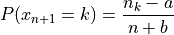
Suppose there are n samples occupying m tables. Then the probability that the n+1 sample occupies table 1 <= k <= m is:
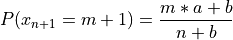
and the probability that the n+1 sample occupies the new table m+1 is:
The probability of a configuration in which a restaurant contains n customers at m tables, with n_k customers at table k is:
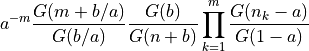
where G is the Gamma function.
Improving running time
Several people have been running this code on larger data sets, and long running times have become a problem.
The “right thing” would be to rewrite the code to make it run efficiently, but until someone gets around to doing that, I’ve added very simple multi-threading support using OpenMP.
To compile wordseg-ag with OpenMP support, use the AG_PARALLEL option for cmake:
cmake -DAG_PARALLEL=ON ..
On my 8 core desktop machine, the multi-threaded version runs about twice as fast as the single threaded version, albeit using on average about 6 cores (i.e., its parallel efficiency is about 33%).
Quadruple precision
On very long strings the probabilities estimated by the parser can sometimes underflow, especially during the first couple of iterations when the probability estimates are still very poor.
The right way to fix this is to rewrite the program so it rescales all of its probabilities during the computation to avoid unflows, but until someone gets around to doing this, I’ve implemented a hack, which is just to compile the code using new new quadruple-precision floating point maths.
To compile wordseg-ag on quadruple float precision, use the AG_QUADRUPLE option for cmake:
cmake -DAG_QUADRUPLE=ON ..
Information on DIBS provided by original contributor
A DiBS model assigns, for each phrase-medial diphone, a value between 0 and 1 inclusive (representing the probability the model assigns that there is a word-boundary there). In practice, these probabilities are mapped to hard decisions, with the optimal threshold being 0.5.
Without any training at all, a phrasal-DiBS model can assign sensible defaults (namely, 0, or the context-independent probability of a medial word boundary, which will always be less than 0.5, and so effectively equivalent to 0 in a hard-decisions context). The outcome in this case would be total undersegmentation (for default 0; total oversegmentation for default 1).
It takes relatively little training to get a DiBS model up to near-ceiling (i.e. the model’s intrinsic ceiling: “as good as that model will get even if you train it forever”, rather than “perfect for that dataset”). Moreover, in principle you can have the model do its segmentation for the nth sentence based on the stats it has accumulated for every preceding sentence (and with a little effort, even on the nth sentence as well). In practice, since I was never testing on the training set for publication work, but I was testing on huge test sets, I optimized the code for mixed iterative/batch training, meaning it could read in a training set, update parameteres, test, and then repeat ad infinitum.