Gaussians

This example illustrates ABX discriminability on the simplest possible classes: samples drawn from Gaussians. We start in 2D for visual intuition, then move to 1D where the ABX score admits a closed form and we can check fastabx against the theoretical value.

Throughout, we use the Euclidean distance.

import math

import matplotlib.pyplot as plt
import numpy as np

from fastabx import Dataset, Score, Task

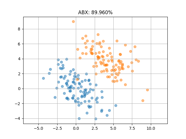
Two 2D Gaussians

We draw two clusters from \(\mathcal{N}(\mu_A, \Sigma)\) and \(\mathcal{N}(\mu_B, \Sigma)\) with a shared (correlated) covariance and a fixed diagonal shift between the means. The reported ABX score is the probability that a probe drawn from class \(A\) ends up closer to another class-\(A\) sample than to a class-\(B\) sample.

n = 100
diagonal_shift = 4
mean = np.zeros(2)
cov = np.array([[4, -2], [-2, 3]])

rng = np.random.default_rng(seed=0)
first = rng.multivariate_normal(mean, cov, n)
second = rng.multivariate_normal(mean + np.ones(2) * diagonal_shift, cov, n)

dataset = Dataset.from_numpy(np.vstack([first, second]), {"label": [0] * n + [1] * n})
task = Task(dataset, on="label")
score = Score(task, "euclidean")

plt.scatter(*first.T, alpha=0.5)
plt.scatter(*second.T, alpha=0.5)
plt.axis("equal")
plt.grid()
plt.title(f"ABX: {1 - score.collapse():.3%}")
plt.show()

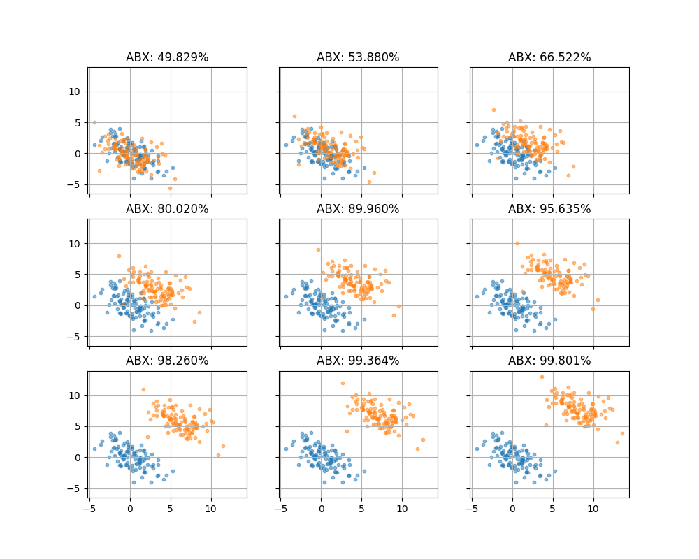
Two 2D Gaussians with increasing shift

Now we keep the same covariance for both classes and sweep the displacement between their means along the diagonal. The score climbs from chance level (fully overlapping clouds) up toward \(1\) as the clusters separate.

n = 100
shift = np.ones(1)
mean = np.zeros(2)
cov = np.array([[4, -2], [-2, 3]])

rng = np.random.default_rng(seed=0)
first = rng.multivariate_normal(mean, cov, n)
second = rng.multivariate_normal(mean, cov, n)

fig, axes = plt.subplots(figsize=(10, 8), nrows=3, ncols=3, sharex=True, sharey=True)
for ax in axes.flatten():
    dataset = Dataset.from_numpy(np.vstack([first, second]), {"label": [0] * n + [1] * n})
    task = Task(dataset, on="label")
    score = Score(task, "euclidean")

    ax.scatter(*first.T, s=10, alpha=0.5)
    ax.scatter(*second.T, s=10, alpha=0.5)
    ax.grid()
    ax.set_title(f"ABX: {1 - score.collapse():.3%}")
    second += shift

plt.show()

Closed-form ABX for two 1D Gaussians

In 1D with a shared variance, the ABX score can be written in closed form, which makes it a good sanity check for the implementation. Let \(A = \mathcal{N}(\mu_a, \sigma^2)\) and \(B = \mathcal{N}(\mu_b, \sigma^2)\), and write the normalized separation \(t = (\mu_a - \mu_b) / \sigma\). Then

\[\mathrm{ABX}(A, B) \;=\; \mathbb{P}\bigl(|x-a| < |x-b|\bigr) \;=\; \frac{1}{2} + \frac{1}{2}\,\operatorname{erf}\!\left(\frac{t}{2}\right)\operatorname{erf}\!\left(\frac{t}{2\sqrt{3}}\right),\]

where \(a \sim A\), \(x \sim A\), \(b \sim B\) are mutually independent. The result depends only on \(t\): it equals \(\tfrac{1}{2}\) at \(t = 0\), tends to \(1\) as \(|t| \to \infty\), and is symmetric under \(\mu_a \leftrightarrow \mu_b\).

Derivation

Step 1: reduce the event to a product of two Gaussians. Both distances are nonnegative, so squaring preserves the inequality:

\[|x-a| < |x-b| \iff (x-a)^2 < (x-b)^2.\]

Expanding, cancelling \(x^2\), and factoring gives

\[(a-b)(a+b-2x) < 0.\]

Introducing \(U = a-b\) and \(V = a+b-2x\),

\[\mathbb{P}\bigl(|x-a|<|x-b|\bigr) = \mathbb{P}(UV < 0).\]

Step 2: joint distribution of \(U\) and \(V\) . Both are linear combinations of independent Gaussians, hence jointly Gaussian. With \(m = \mu_a - \mu_b\),

\[\mathbb{E}[U] = m, \qquad \mathbb{E}[V] = -m,\]

\[\operatorname{Var}(U) = 2\sigma^2, \qquad \operatorname{Var}(V) = 6\sigma^2,\]

\[\operatorname{Cov}(U,V) = \operatorname{Cov}(a,a) - \operatorname{Cov}(b,b) = 0.\]

Zero covariance for jointly Gaussian variables implies independence:

\[U \sim \mathcal{N}(m,\,2\sigma^2), \qquad V \sim \mathcal{N}(-m,\,6\sigma^2), \qquad U \perp V.\]

Step 3: factor the probability. For independent \(U, V\),

\[\mathbb{P}(UV < 0) = \mathbb{P}(U>0)\mathbb{P}(V<0) + \mathbb{P}(U<0)\mathbb{P}(V>0).\]

With \(p = \mathbb{P}(U>0)\) and \(q = \mathbb{P}(V>0)\), this rearranges to

\[\mathbb{P}(UV<0) = p + q - 2pq = \tfrac{1}{2} - 2\bigl(p-\tfrac{1}{2}\bigr)\bigl(q-\tfrac{1}{2}\bigr).\]

Step 4: evaluate. For \(W \sim \mathcal{N}(\mu_W, \sigma_W^2)\),

\[\mathbb{P}(W>0) - \tfrac{1}{2} = \tfrac{1}{2}\,\operatorname{erf}\!\left(\frac{\mu_W}{\sqrt{2}\,\sigma_W}\right).\]

Applied to \(U\) (\(\sigma_U = \sqrt{2}\,\sigma\)) and \(V\) (\(\sigma_V = \sqrt{6}\,\sigma\), \(\mu_V = -m\)),

\[p - \tfrac{1}{2} = \tfrac{1}{2}\,\operatorname{erf}\!\left(\frac{m}{2\sigma}\right), \qquad q - \tfrac{1}{2} = -\tfrac{1}{2}\,\operatorname{erf}\!\left(\frac{m}{2\sqrt{3}\,\sigma}\right),\]

using \(\sqrt{2}\cdot\sqrt{6} = 2\sqrt{3}\) and \(\operatorname{erf}(-z) = -\operatorname{erf}(z)\). Substituting back,

\[\mathbb{P}(UV<0) = \tfrac{1}{2} + \tfrac{1}{2}\,\operatorname{erf}\!\left(\frac{m}{2\sigma}\right)\operatorname{erf}\!\left(\frac{m}{2\sqrt{3}\,\sigma}\right).\]

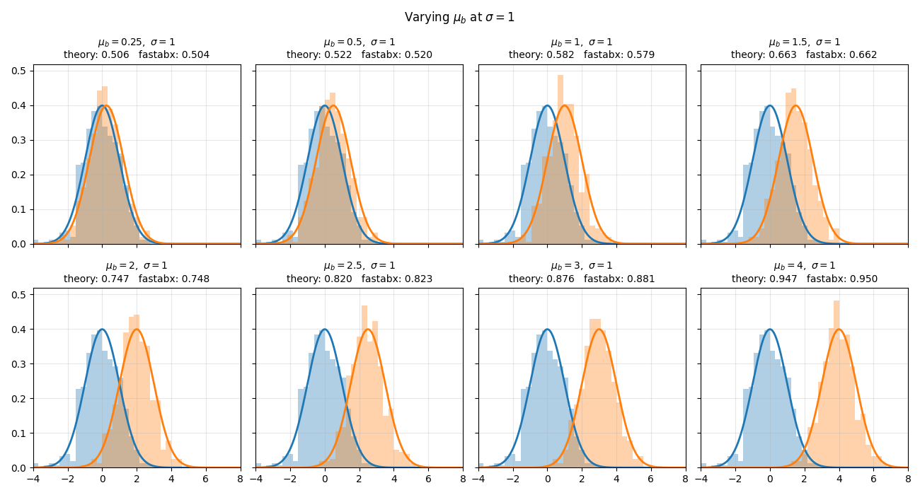
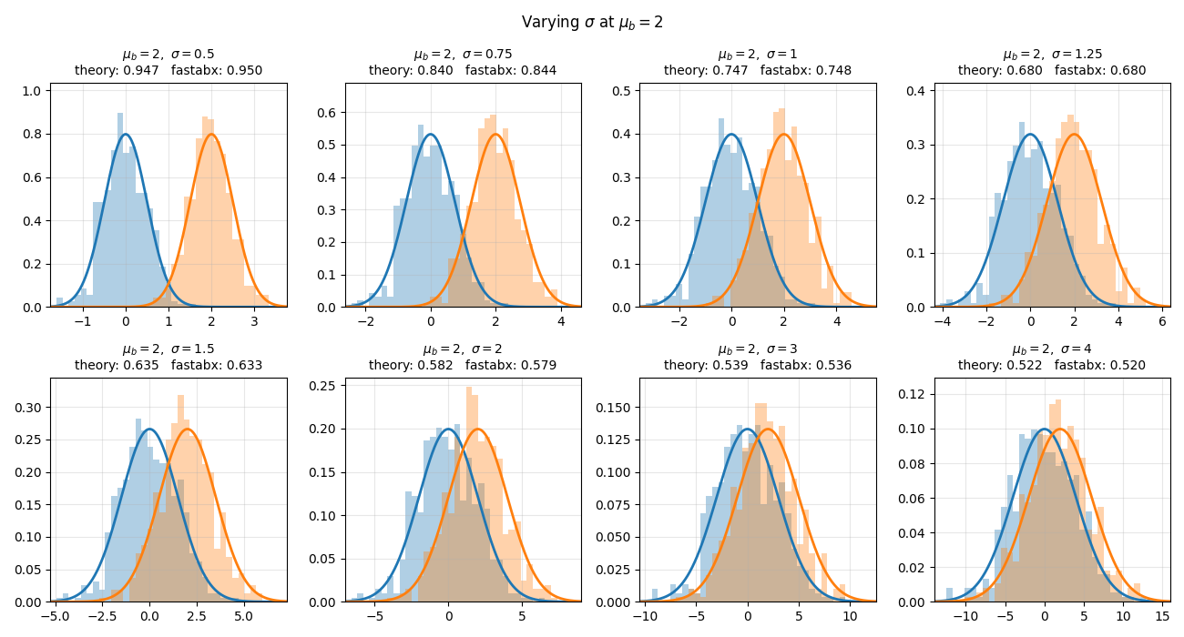
Empirical vs theoretical ABX in 1D

We can now check the formula above against fastabx. The helpers below sample \(n = 500\) points from each class, compute the empirical ABX with Score(Task(...)), and compare it to theoretical_abx. Each panel overlays the true densities and the sample histograms, with the two scores shown in the title. We then sweep one parameter at a time: \(\mu_b\) at fixed \(\sigma\), then \(\sigma\) at fixed \(\mu_b\).

def theoretical_abx(mu_a: float, mu_b: float, sigma: float) -> float:
    """Closed-form ABX score for two 1D Gaussians with shared variance."""
    t = (mu_a - mu_b) / sigma
    return 0.5 + 0.5 * math.erf(t / 2) * math.erf(t / (2 * math.sqrt(3)))


def empirical_abx(a: np.ndarray, b: np.ndarray) -> float:
    """Empirical ABX score on two 1D samples computed with ``fastabx``."""
    features = np.concatenate([a, b]).reshape(-1, 1)
    labels = {"label": [0] * len(a) + [1] * len(b)}
    dataset = Dataset.from_numpy(features, labels)
    return 1.0 - Score(Task(dataset, on="label"), "euclidean").collapse()


def gaussian_pdf(x: np.ndarray, mu: float, sigma: float) -> np.ndarray:
    """Density of the normal distribution with mean ``mu`` and standard deviation ``sigma``."""
    return np.exp(-0.5 * ((x - mu) / sigma) ** 2) / (sigma * math.sqrt(2 * math.pi))


def plot_panel(
    ax: plt.Axes,
    mu_a: float,
    mu_b: float,
    sigma: float,
    x_range: tuple[float, float] | None,
    n: int,
    seed: int,
) -> None:
    """Draw one panel comparing the theoretical and empirical ABX scores."""
    rng = np.random.default_rng(seed)
    a = rng.normal(mu_a, sigma, n)
    b = rng.normal(mu_b, sigma, n)
    if x_range is None:
        pad = 3.5 * sigma
        lo, hi = min(mu_a, mu_b) - pad, max(mu_a, mu_b) + pad
    else:
        lo, hi = x_range
    grid = np.linspace(lo, hi, 400)
    bins = np.linspace(lo, hi, 40).tolist()

    ax.hist(a, bins=bins, density=True, alpha=0.35, color="C0")
    ax.hist(b, bins=bins, density=True, alpha=0.35, color="C1")
    ax.plot(grid, gaussian_pdf(grid, mu_a, sigma), color="C0", lw=2)
    ax.plot(grid, gaussian_pdf(grid, mu_b, sigma), color="C1", lw=2)
    ax.set_xlim(lo, hi)
    peak = 1.0 / (sigma * math.sqrt(2 * math.pi))
    ax.set_ylim(0, 1.3 * peak)
    ax.grid(alpha=0.3)

    theory = theoretical_abx(mu_a, mu_b, sigma)
    empirical = empirical_abx(a, b)
    ax.set_title(
        rf"$\mu_b={mu_b:g},\ \sigma={sigma:g}$" + "\n" + f"theory: {theory:.3f}   fastabx: {empirical:.3f}",
        fontsize=10,
    )

Varying the mean separation (fixed \(\sigma = 1\), \(\mu_a = 0\))

n = 500
seed = 0
mu_a = 0.0
sigma = 1.0
mu_bs = [0.25, 0.5, 1.0, 1.5, 2.0, 2.5, 3.0, 4.0]
x_range = (-4.0, 8.0)

fig, axes = plt.subplots(figsize=(13, 7), nrows=2, ncols=4, sharex=True, sharey=True)
for ax, mu_b in zip(axes.flatten(), mu_bs, strict=True):
    plot_panel(ax, mu_a, mu_b, sigma, x_range, n, seed)
fig.suptitle(rf"Varying $\mu_b$ at $\sigma={sigma:g}$")
fig.tight_layout()
plt.show()

Varying the standard deviation (fixed \(\mu_a = 0\), \(\mu_b = 2\))

n = 500
seed = 0
mu_a = 0.0
mu_b = 2.0
sigmas = [0.5, 0.75, 1.0, 1.25, 1.5, 2.0, 3.0, 4.0]

fig, axes = plt.subplots(figsize=(13, 7), nrows=2, ncols=4)
for ax, sigma in zip(axes.flatten(), sigmas, strict=True):
    plot_panel(ax, mu_a, mu_b, sigma, None, n, seed)
fig.suptitle(rf"Varying $\sigma$ at $\mu_b={mu_b:g}$")
fig.tight_layout()
plt.show()